
Modern vehicles are rolling networks. Powertrain, chassis, body control, infotainment, ADAS, and even seats speak through shared data lines. If you build, test, or service electronic control units (ECUs), you’ll run into Controller Area Network (CAN). This article gives a clear, field-ready Introduction to CAN bus for automotive—from signaling and arbitration to hardware choices, timing math, diagnostics, and design tips that matter in labs and on the road. If your pcb design or firmware touches anything on wheels, this is the backbone you need to understand.
What is the CAN bus?
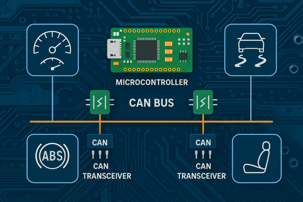
CAN is a multi-master, message-oriented protocol designed by Bosch in the 1980s for robust communication in harsh environments. Multiple nodes share a two-wire differential link (CAN_H and CAN_L). Any node may transmit when the bus is idle. A hardware-level arbitration scheme guarantees that only one node talks at a time, and the message with the highest priority wins without wasting bandwidth. Messages are identified by an ID, not a destination address. Every ECU on the network receives every frame and decides in hardware or software whether to accept it (filtering by ID) or ignore it. This publish-subscribe model scales very well: adding a new device that logs RPM or reads throttle position does not require rewriting every other module—just subscribe to the relevant IDs. CAN runs over twisted pair with recessive (logical 1) and dominant (logical 0) states. Electrical robustness is part of its appeal: common-mode noise rejection, fault confinement, error counters, and automatic retransmission keep data flowing even when the environment gets noisy or a connector is less than perfect.
Basic frame structure and arbitration
A classical CAN 2.0 frame includes these fields in order: Start of Frame (SOF), Arbitration field (identifier + RTR), Control field (DLC), Data field (0..8 bytes), CRC, ACK slot, and End of Frame (EOF). There are two frame formats: Base (11-bit ID) and Extended (29-bit ID using an extended identifier field and IDE bit). Arbitration is the signature feature. CAN uses wired-AND logic (dominant = 0 overrides recessive = 1). Multiple nodes may begin transmitting at the same time. Bit by bit, any node that transmits a recessive 1 but reads back a dominant 0 detects a loss of arbitration and immediately stops, leaving the highest-priority message (lowest numeric ID) to continue without corruption. No time is lost on collisions. This makes scheduling predictable and keeps latency small for safety-critical traffic. The Data Length Code (DLC) in the control field encodes payload length for classical CAN (0..8 bytes). In CAN FD, DLC maps to up to 64 bytes. The ACK slot allows any receiver to signal correct receipt by driving a dominant 0; the transmitter monitors this and can retry if no ACK is detected.
Bit timing and baud rates
CAN transmits using non-return-to-zero (NRZ) coding with bit stuffing: after five identical bits, a complementary stuff bit is inserted to keep edges coming for synchronization. Each bit time is divided into segments: SYNC_SEG, PROP_SEG, PHASE_SEG1, and PHASE_SEG2. The sum of these defines the Time Quanta (Tq) count per bit. Key parameters you’ll see in datasheets and drivers are Baud Rate Prescaler (BRP), TSEG1 (PROP+PH1), TSEG2 (PH2), and SJW (resynchronization jump width). Practical steps for timing setup: 1) Choose the bus rate (e.g., 500 kbit/s for powertrain), 2) Derive a time-quanta clock from the peripheral clock using BRP, 3) Set TSEG1 and TSEG2 so the sample point lands around 80% (common automotive target), 4) Pick SJW = 1..4 Tq to tolerate jitter, 5) Validate on hardware with a CAN analyzer and a scope. Common classical CAN speeds: 125 kbit/s (body), 250 kbit/s (heavy-duty/J1939), 500 kbit/s (powertrain), 1 Mbit/s (short harness). CAN FD splits timing into two phases: arbitration at a classic rate and data phase up to 2, 4, 5, or even 8 Mbit/s on short, well-terminated segments. Sampling at 80% is a good starting point, but some stacks default to 75–87.5%; match your transceiver and harness length. If communication seems marginal, try nudging the sample point later (larger TSEG1) to tolerate long cable propagation.
CAN transceivers and isolation
The CAN controller in your MCU speaks digital logic; a transceiver translates this to the differential physical layer and vice versa. Automotive-grade transceivers include protections for ESD, short to battery/ground, thermal shutdown, and passive/active fail-safe states. Key choices: • Common-mode voltage range and input thresholds: pick parts tolerant to ±12 V transients and relatable to your system ground. • Loop delay symmetry: tighter specs help timing margins at high bit rates and with long cables. • Low-power/silent modes: many transceivers support standby and partial networking to cut ignition-off current. • High-speed vs fault-tolerant: ISO 11898-2 for high speed; fault-tolerant (ISO 11898-3) tolerates single-wire operation at lower speeds in body networks. Galvanic isolation is common for aftermarket tools and for noisy domains (e.g., high-voltage EV battery packs). Isolated CAN transceivers or digital isolators plus a standard transceiver protect low-voltage logic from high common-mode disturbances and break ground loops. In safety-related designs, isolation helps partition functional safety domains and improve EMC. For pcb design, place the transceiver close to the bus connector, keep CAN_H/CAN_L as a controlled-impedance differential pair with tight coupling, and use a solid reference under the pair. Add ESD diodes near the connector, keep stub lengths short, and route away from high-dv/dt nodes (e.g., motor phase edges or DC-DC switch nodes).
Error detection and fault confinement
Reliability is baked into CAN. Error detection covers: • Bit monitoring: every transmitter monitors the bus and detects mismatches. • Bit stuffing check: receivers verify proper removal of inserted bits. • CRC: a frame-level cyclic redundancy check detects burst errors. • Form and ACK errors: receivers flag malformed segments and missing acknowledgments. On any error, a node transmits an error frame (dominant) to abort the current message so all nodes discard it. Each controller maintains Transmit Error Counter (TEC) and Receive Error Counter (REC). These drive fault confinement states: • Error-active: normal operation; error flags are active-state. • Error-passive: after counters exceed a threshold; node still participates but sends passive error flags (recessive). • Bus-off: after severe errors; the node is forced silent. Recovery from bus-off requires a defined idle time or software reset depending on the controller. This built-in self-healing behavior is why CAN works well with intermittent faults, loose connectors, or a failing module. You get graceful degradation instead of network chaos.
Common CAN topologies
The recommended physical layout for high-speed CAN is a linear bus with 120 Ω termination at both extreme ends. The equivalent parallel resistance is 60 Ω. Stubs should be very short—ideally under 0.3 m at 500 kbit/s and much shorter at 1 Mbit/s—to limit reflections. Good practices: • Twisted pair cabling with 90 Ω differential impedance • Keep total bus length matched to the data rate (e.g., 40 m at 500 kbit/s is common in vehicles; much longer is possible at 125 kbit/s) • Place terminations at the harness extremes, not in the middle • Use common-mode chokes and RC filters near the connector if EMC testing shows radiated emissions peaks Variants: Star and multiple stars are sometimes used in body networks at low speeds, but reflection management becomes tricky. For maintenance or retrofit, backbone with short drops works if you respect stub length guidance. EVs introduce strong EMI sources; a well-routed, tightly coupled pair and shielded cable in aggressor areas can make all the difference.
High-speed vs low-speed CAN
High-speed CAN (ISO 11898-2) runs up to 1 Mbit/s (arbitration phase for FD) using a two-wire differential pair with 120 Ω terminations. It’s used for powertrain, chassis, and safety functions. Fault-tolerant/low-speed CAN (ISO 11898-3) is popular in body electronics. It supports lower data rates (up to ~125 kbit/s), can continue operating in single-wire mode if one line is shorted, and often uses different termination rules. Trade-offs: • High-speed = higher bandwidth, tighter wiring rules • Low-speed = better resilience to physical faults, lower bandwidth, simplified harnessing in some cases When planning a vehicle architecture, many OEMs mix networks: a high-speed backbone for time-sensitive traffic and low-speed segments for non-urgent functions.
CAN FD and future extensions
CAN FD (ISO 11898-1:2015) extends classical CAN with: • Data field up to 64 bytes • Two bit rates: classic arbitration phase and faster data phase (BRS bit) • Larger CRC to keep error detection strength despite longer frames • Optional Error State Indicator (ESI) to expose the transmitter’s error-passive status Benefits: fewer frames for bulk payloads, shorter transfer time at high data rates, and lower CPU interrupt load. Examples: firmware updates, deep sensor packets, logging raw ADC data, or gatewaying between domains. Looking forward, you’ll also see CAN XL discussions in industry groups: aiming for higher throughput over similar media and larger payloads while keeping deterministic arbitration. For many automotive and off-highway applications, CAN FD already hits a sweet spot between cost, tooling, and performance.
Implementing CAN in microcontrollers
MCUs from NXP, Infineon, ST, Microchip, Renesas, TI, Espressif, and others offer integrated CAN/CAN FD controllers. Implementation steps that consistently lead to reliable results: 1) Pin mux and clocks: Select CAN TX/RX pins with shortest routes to the transceiver. Provide a stable peripheral clock that supports your timing targets. 2) Bit timing: Compute BRP, TSEG1, TSEG2, SJW for your desired sample point; verify with a logic analyzer. 3) Filters and masks: Configure acceptance filters to queue only relevant frames, lowering CPU load. Many controllers support list, mask-based, and range filters. 4) Interrupts and DMA: Use separate RX and TX mailboxes/queues. Enable FIFO and DMA if available to reduce ISR time. 5) Error handling: Register callbacks for error-active to error-passive transitions, bus-off entry, and restart logic. Log TEC/REC values for field diagnostics. 6) Low-power modes: Use wake-up on bus activity or selective wake for quiescent systems. 7) CAN FD specifics: Configure nominal and data bit timing separately. Start with a moderate data bit rate (e.g., 2 Mbit/s) and verify signal integrity before pushing higher. 8) Bootloader considerations: For over-the-bus firmware updates, guard against partial writes; use signatures and power-loss recovery.
Debugging and testing with CAN tools
A solid toolkit saves days: • USB or Ethernet CAN interfaces: Peak, Kvaser, Vector, NI, and many others; choose drivers supported by your OS and scripting language. • Software: Bus analyzers can record, filter, replay, and graph messages. Features to value: timestamp precision, trigger conditions, error frame capture, and database (DBC/ARXML) support. • DBC files: Map raw IDs and signals to human-readable names, bit positions, scaling, and units. This turns 0x0CFF0500 into “Engine Speed = 742 rpm” in graphs and logs. • Oscilloscope: Check recessive/dominant levels, differential swing (~2 V), and ringing at edges. Verify termination and look for long stubs by watching reflections. • Signal integrity checks: With CAN FD, check eye openings and symmetry. A slightly late sample point may fix marginal links. • Conformance and EMC: If your product goes into vehicles, budget lab time for immunity and emissions tests early—radiated peaks near bit edges are common and can be tamed with chokes, common-mode filters, and cleaner return paths. For production, add end-of-line tests: basic loopback, filter checks, and bus-off recovery. If your ECU will be serviced in the field, design in a debug header for CAN access, or expose CAN on an existing service connector where allowed.
Applications beyond automotive
CAN’s reliability, cost, and tooling spread far beyond cars. Examples: • Heavy-duty and agriculture: J1939 atop CAN for trucks, buses, tractors, harvesters. • Marine: NMEA 2000 for boats and yachts. • Industrial: CANopen/DeviceNet for motion control, sensors, and drives. • Medical: hospital beds, pumps, imaging gantries. • Robotics and mobility: wheel modules, motor controllers, battery packs. The same skills and test habits carry across domains.
Wiring, termination, and EMC tips (hardware you can ship)
- Termination: Two 120 Ω resistors at the ends only. On modular harnesses, use switchable or plug-in terminators so service teams can verify with a multimeter (expect ~60 Ω end-to-end with power off). 2) Stubs: Keep them short. If a T-connector must be used, verify reflections on a scope at the highest data rate. 3) Common-mode chokes: Place near the connector; they suppress radiated emissions without hurting differential signaling much. 4) ESD/TVS: Fast diodes to ground or a bidirectional TVS to clamp to safe levels. Size for ISO pulsed surge profiles if required by your market. 5) Shielding: Use shielded twisted pair in noisy zones (traction inverters, DC-DC converters). Terminate the shield to chassis with low impedance (spring fingers, 360° clamps). 6) Connectors: Automotive-grade sealed connectors with positive latches; align pinouts so CAN_H/CAN_L stay adjacent to preserve coupling. 7) Grounding: Provide a short, low-impedance return for ESD and transient currents; keep it out of sensitive analog grounds. 8) Power: Decouple transceivers locally and consider reverse-battery protection on the supply.
Software design patterns that save you pain
• Message catalog: Keep a single source of truth for IDs, signal locations, scaling, endianness, and units. Generate C headers and Python/Matlab mappings from it. • RTOS mailboxes: Separate RX parsing from application logic; use queues to avoid blocking. • Rate-monotonic scheduling: Transmit periodic frames with jitter budgets; use event-driven sends for infrequent signals. • Health monitoring: Add counters for timeouts on critical signals (e.g., vehicle speed). Trigger limp modes if missing. • Bootloader updates: Chunked transfers with CRC; resume after interruption; prevent downgrades unless explicitly permitted. • Security basics: Classical CAN has no authentication; do not put sensitive functions on unprotected buses. Use secure gateways, seed-key access control, and cryptographically signed updates.
Safety and functional safety notes
If your ECU affects steering, braking, or torque, treat CAN timing and error handling with the same rigor as the control algorithms. Useful habits: • Arbitration priority: Assign lower numeric IDs to signals with tighter latency budgets. • Redundancy: For safety signals, consider dual-path communication or periodic alive counters plus CRC on the payload. • Diagnostics: Implement DTCs for bus-off events, ACK errors, and message timeouts. • HIL testing: Hardware-in-the-loop setups reveal race conditions and timing edges that unit tests won’t show.
Addressing CAN security risks
Classical CAN was not built with authentication or encryption. Modern vehicles mitigate this with segmented networks, secure gateways, application-level message counters/CRC, and diagnostic access control. Good practice for new products: • Gate sensitive commands behind authenticated sessions. • Enforce sanity checks on all actuator commands. • Log unusual traffic patterns and rate-limit control messages. • If you bridge Ethernet or wireless to CAN, harden that bridge—most attacks target the bridge.
From prototype to product: a checklist
• Define IDs and timing budgets early; avoid later remaps that ripple through all nodes. • Lock down naming and scaling for signals; keep a versioned DBC. • Pick a transceiver with the right protections; place it near the connector; route the pair as a tight differential. • Validate bit timing with a scope/analyzer on the exact harness you will ship. • Add test points for CAN_H and CAN_L, and a header for a probe or service tool. • Pre-qualify EMC in-house with a current probe and near-field sniffers. • Document your bus error handling and bus-off recovery rules.
Worked timing example (practical numbers)
Goal: 500 kbit/s classical CAN on a 40 m harness. Suppose your MCU has a 80 MHz CAN peripheral clock. Choose BRP = 10 → time-quanta clock = 8 MHz (125 ns per Tq). Pick 16 Tq per bit (16 × 125 ns = 2 μs → 500 kbit/s). Set TSEG1 = 12 Tq, TSEG2 = 3 Tq, SYNC_SEG = 1 Tq → sample point = (1 + 12) / 16 = 81.25%. SJW = 2 Tq. Measure on a scope: differential swing near 2 V for dominant, minimal ringing, no over/undershoot beyond transceiver limits. If margins look tight, move the sample point to 85% by shifting one Tq from TSEG2 to TSEG1 and retest.
When to choose CAN FD in a new design
Pick CAN FD when: • You need payloads beyond 8 bytes or frequent bursts (sensors with dense data, over-the-air updates over CAN, logging). • You control the whole network or know all nodes support FD. • Harness lengths are moderate and you can validate signal integrity at higher data rates. Stay with classical CAN when: • You’re adding to an existing network with legacy modules. • Bandwidth needs are low and simplicity is valuable. • You cannot re-qualify EMC at higher edge rates right now. A hybrid path is common: set arbitration at 500 kbit/s and data at 2 Mbit/s, use FD only for selected frames, and keep classical timing for safety-critical traffic.
Interfacing with diagnostics and OBD-II
Passenger cars expose a standardized OBD-II connector. While the diagnostic layer (UDS, ISO-TP) sits above CAN, understanding CAN basics helps during root-cause analysis. For developers of tools or aftermarket modules: • Respect OEM policies and legal requirements for safety systems. • Keep passive sniffing as the default mode; transmit only when needed and with rate limits. • For ISO-TP flows, budget memory for reassembly and timeouts.
Real-world failure cases and how to solve them
• Missing termination: The bus measures ~120 Ω instead of ~60 Ω and frames show ringing or frequent CRC errors. Fix: Add the second 120 Ω at the far end. • Long stubs: Intermittent errors at higher rates, improves at 125 kbit/s. Fix: Relocate the node, shorten the drop, or move the termination. • Ground offsets: Repeated errors near high-current returns. Fix: Better bonding, isolation, or reroute CAN away from noisy grounds. • Tool overload: USB interfaces dropping frames during bursts. Fix: Hardware timestamping, higher-performance interface, or throttled logging. • ECU brownout: Node reboots during crank and floods the bus with error frames. Fix: Hold-up capacitance, brownout reset, and rate-limited startup chatter.
Putting it all together
CAN remains the heartbeat of vehicle communication. The electrical layer is tough, arbitration gives deterministic behavior under heavy load, and the ecosystem of tools and MCUs is mature. Whether you’re tuning timing registers, laying out a transceiver footprint, or decoding DBC signals for data science, the same fundamentals apply: clean wiring, correct bit timing, thoughtful ID assignments, and disciplined testing.
Conclusion
If you work on automotive electronics, mastery of CAN pays off quickly. Start with a solid transceiver and tidy harness, get timing right with a scope and analyzer, filter aggressively in software, and treat error handling as a first-class feature. As projects scale, CAN FD gives you more payload and speed without throwing away hard-won knowledge. With careful planning and repeatable tests, your ECUs will talk reliably for years, even in punishing environments.