
A PID controller (Proportional-Integral-Derivative controller) is a fundamental component in control systems, widely used in industrial automation, robotics, and various other applications. This article delves into the intricacies of PID controllers, from their basic principles to advanced tuning techniques, providing a comprehensive understanding of their role in modern control systems.
What is a PID Controller?
A PID controller is a control loop feedback mechanism commonly used in industrial control systems. It continuously calculates an error value as the difference between a desired setpoint and a measured process variable, applying a correction based on proportional, integral, and derivative terms.
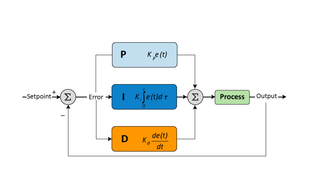
The PID controller algorithm can be expressed mathematically as:
u(t)=Kpe(t)+Ki∫0te(τ)dτ+Kdde(t)dtu(t) = K_p e(t) + K_i \int_{0}^{t} e(\tau) d\tau + K_d \frac{de(t)}{dt}u(t)=Kpe(t)+Ki∫0te(τ)dτ+Kddtde(t)
where:
- u(t)u(t)u(t) is the control output.
- e(t)e(t)e(t) is the error between the setpoint and the process variable.
- KpK_pKp is the proportional gain.
- KiK_iKi is the integral gain.
- KdK_dKd is the derivative gain.
What are the Components of PID Control?
1. Proportional (P) Control:
The proportional term produces an output value that is proportional to the current error value. The proportional response can be adjusted by multiplying the error by a constant KpK_pKp, known as the proportional gain.
up(t)=Kpe(t)u_p(t) = K_p e(t)up(t)=Kpe(t)
A high proportional gain results in a large change in the output for a given change in error, which can lead to a faster response. However, if KpK_pKp is too high, the system can become unstable and oscillate.
2. Integral (I) Control:
The integral term is concerned with the accumulation of past errors. If the error has been present for a long time, the integral term grows, increasing the control output to eliminate the residual steady-state error that a proportional controller cannot correct.
ui(t)=Ki∫0te(τ)dτu_i(t) = K_i \int_{0}^{t} e(\tau) d\tauui(t)=Ki∫0te(τ)dτ
Integral control is essential for systems where a steady-state error must be eliminated, but excessive integral action can lead to overshoot and instability.
3. Derivative (D) Control:
The derivative term predicts future error based on its rate of change. By taking the derivative of the error, the controller anticipates the system’s behavior and applies a corrective action accordingly.
ud(t)=Kdde(t)dtu_d(t) = K_d \frac{de(t)}{dt}ud(t)=Kddtde(t)
Derivative control can improve the stability and response time of the system by damping the oscillations caused by the proportional and integral terms. However, it is sensitive to noise in the error signal and can lead to erratic control actions if not tuned properly.
PID Controller Tuning
Tuning a PID controller involves adjusting the KpK_pKp, KiK_iKi, and KdK_dKd parameters to achieve the desired system response. Several methods can be employed for PID tuning:
1. Manual Tuning:
Manual tuning involves iteratively adjusting the gains and observing the system’s response. This method requires experience and intuition about the system’s dynamics.
2. Ziegler-Nichols Method:
The Ziegler-Nichols method is a heuristic approach to tuning PID controllers. It involves setting the integral and derivative gains to zero, increasing the proportional gain until the system oscillates with a constant amplitude (critical gain KuK_uKu), and then setting the gains based on the oscillation period TuT_uTu:
- Kp=0.6KuK_p = 0.6 K_uKp=0.6Ku
- Ki=1.2Ku/TuK_i = 1.2 K_u / T_uKi=1.2Ku/Tu
- Kd=3KuTu/40K_d = 3 K_u T_u / 40Kd=3KuTu/40
3. Cohen-Coon Method:
The Cohen-Coon method is another heuristic tuning approach that provides better performance for systems with significant time delays. It involves setting the gains based on the system’s response to a step input.
4. Software-Based Tuning:
Modern control systems often use software tools for automatic PID tuning. These tools employ algorithms that adjust the gains based on the system’s response to test signals, providing optimal tuning parameters with minimal manual intervention.
PID Controller Problem Example
Consider a temperature control system for an industrial furnace. The objective is to maintain the furnace temperature at a desired setpoint, despite disturbances and changes in the heating load.
Step 1: Define the System Dynamics
The system can be modeled as a first-order process with a time delay:
dT(t)dt+aT(t)=bH(t−τ)\frac{dT(t)}{dt} + aT(t) = bH(t-\tau)dtdT(t)+aT(t)=bH(t−τ)
where T(t)T(t)T(t) is the furnace temperature, H(t)H(t)H(t) is the heating input, aaa and bbb are system parameters, and τ\tauτ is the time delay.
Step 2: Implement the PID Controller
The PID controller adjusts the heating input based on the temperature error:
H(t)=Kpe(t)+Ki∫0te(τ)dτ+Kdde(t)dtH(t) = K_p e(t) + K_i \int_{0}^{t} e(\tau) d\tau + K_d \frac{de(t)}{dt}H(t)=Kpe(t)+Ki∫0te(τ)dτ+Kddtde(t)
Step 3: Tune the Controller
Using the Ziegler-Nichols method, the critical gain KuK_uKu and oscillation period TuT_uTu are determined experimentally. The PID gains are then set based on these values.
Step 4: Simulate and Validate
The system’s response is simulated with the tuned PID controller to ensure that it meets the desired performance criteria, such as minimal overshoot, fast settling time, and zero steady-state error.
What are the Applications of PID Controllers
PID controllers are ubiquitous in various industries and applications:
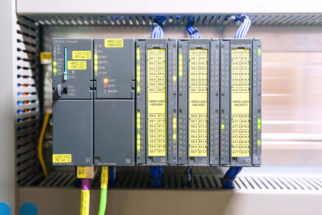
1. Industrial Automation:
PID controllers are extensively used in process control systems for regulating variables such as temperature, pressure, flow, and level in industrial plants.
2. Robotics:
In robotics, PID controllers are used for precise motion control, ensuring accurate positioning and speed regulation of robotic arms and mobile robots.
3. Aerospace:
PID controllers are employed in aerospace applications for controlling the attitude, altitude, and speed of aircraft and spacecraft.
4. Automotive:
Automotive systems utilize PID controllers for engine control, cruise control, and stability control, enhancing vehicle performance and safety.
5. Consumer Electronics:
In consumer electronics, PID controllers are used in devices such as air conditioners, refrigerators, and washing machines to regulate temperature, speed, and other parameters.
What is Loop System in PID Control
A control loop system consists of several components working together to maintain the desired output. The key elements of a PID control loop system include:
1. Sensor:
The sensor measures the process variable (e.g., temperature, pressure) and provides feedback to the controller.
2. Controller:
The PID controller calculates the control output based on the error between the setpoint and the process variable.
3. Actuator:
The actuator implements the control action determined by the controller, adjusting the process to achieve the desired setpoint.
4. Process:
The process is the system being controlled, such as a furnace, motor, or valve.
5. Feedback Loop:
The feedback loop continuously provides the process variable to the controller, enabling real-time adjustments and maintaining the desired output.
Advanced PID Control Techniques
Modern PID controllers incorporate advanced techniques to enhance their performance:
1. Adaptive PID Control:
Adaptive PID controllers automatically adjust their gains in real-time based on changes in the system dynamics, improving performance in varying conditions.
2. Model Predictive Control (MPC):
MPC is a sophisticated control strategy that uses a model of the system to predict future behavior and optimize control actions. It can be combined with PID control for improved performance.
3. Fractional Order PID Control:
Fractional order PID controllers extend the traditional PID control by using fractional calculus, providing greater flexibility and improved control for certain systems.
4. Fuzzy PID Control:
Fuzzy logic can be integrated with PID control to handle nonlinearities and uncertainties in the system, offering robust performance in complex environments.
PID Controller Full Form
The full form of PID is Proportional-Integral-Derivative. Each term in the PID controller plays a crucial role in achieving the desired control performance:
- Proportional: Provides immediate response to the current error.
- Integral: Eliminates steady-state error by considering the cumulative error.
- Derivative: Predicts future error and applies corrective action to dampen oscillations.
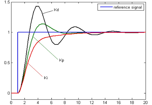
PID Controller Graph
The behavior of a PID controller can be visualized using graphs that show the system’s response over time. Common graphs include:
1. Step Response:
A step response graph shows how the system responds to a sudden change in the setpoint. It helps in analyzing the rise time, overshoot, settling time, and steady-state error.
2. Bode Plot:
A Bode plot represents the frequency response of the system, showing the gain and phase shift as a function of frequency. It is useful for assessing the stability and performance of the control system.
3. Nyquist Plot:
A Nyquist plot displays the system’s response in the complex plane, helping in evaluating the stability and robustness of the control system.
PID Controller Algorithm
The PID controller algorithm involves the following steps:
- Initialize Parameters: Set the initial values of KpK_pKp, KiK_iKi, and KdK_dKd.
- Read Sensor Data: Measure the process variable using the sensor.
- Calculate Error: Compute the error as the difference between the setpoint and the process variable.
- Compute Control Output: Calculate the control output using the PID formula.
- Apply Control Action: Adjust the actuator based on the control output.
- Update State: Update the integral and derivative terms for the next iteration.
- Repeat: Continuously repeat the above steps in real-time.
Conclusion
PID controllers are the backbone of modern control systems, providing robust and efficient control for a wide range of applications. Understanding the principles, tuning methods, and advanced techniques of PID control is essential for designing effective control systems. By leveraging the power of PID controllers, engineers can achieve precise and reliable control, enhancing the performance and stability of industrial processes, robotics, aerospace systems, automotive applications, and consumer electronics.